mdadash.backend.analyses.acf

Autocorrelation Function (ACF)

Classes

ACFAnalysis()	Autocorrelation Function
SlidingWindowACF(u[, physical_property, ...])	Sliding Window ACF

class mdadash.backend.analyses.acf.ACFAnalysis

Bases: WidgetBase

Autocorrelation Function

This widget calculates time-lag autocorrelation for different physical properties.

The following physical properties are supported:

• velocity

• position

• force

A custom SlidingWindowACF is used to calculate autocorrelation of chosen physical property for each new frame against the time-lag buffer / window of past frames.

Important

To correctly compute positional ACF using this widget, you must supply coordinates in the unwrapped convention, also known as no-jump. That is, when atoms pass the periodic boundary, they must not be wrapped back into the primary simulation cell. You can enable NoJump for the universe in the Universe Configuration section in the Settings page of the dashboard.

Inputs

Run mode

The mode in which the widget is run - serial or parallel

Default: serial

Physical property

The physical property to analyze - velocity, position or force

Default: velocity

Selection

The MDAnalysis selection phrase to run this analysis on

Default: all

Dimension type

The desired dimensions to include in the ACF - xyz, xy, yz, xz, x, y or z

Default: xyz

Centered

Use mean subtacted values to calculate ACF

Default: False

Caution

A running updated mean based on data processed so far is used. The number of data samples must be much greater than the lag-time window for this to be accurate

Show running integral

Show running integral of the ACF

Default: False

Tip

Using this option with the velocity physical property, i.e., (VACF) can be used to observe the diffusion coefficient value in the output plot

Show particle ACFs

Show ACFs for individual particles of the selection in the plot

Default: False

Caution

Enabling this option for large selections can slow down the analysis and generation of the plot data

Normalize

Normalize the computed ACF values

Default: False

Custom title

Custom title for the output plot

Default: ‘’

Output

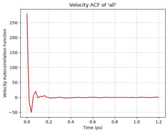
Here is an example output plot of this widget:

Tip

This widget can run in parallel

apply_parallel_results(values)

apply_parallel_results() handler

description = 'Autocorrelation Function'

get_parallel_job()

get_parallel_job() handler

name = 'ACF'

on_input_change(attribute, _old_value, new_value)

on_input_change() handler

on_post_connect()

on_post_connect() handler

on_post_create()

on_post_create() handler

run_every_frame()

run_every_frame() handler

class mdadash.backend.analyses.acf.SlidingWindowACF(u: Universe, physical_property: str = 'velocity', select: str = 'all', dim_type: str = 'xyz', centered: bool = False, show_running_integral: bool = False, show_particle_acfs: bool = False)

Bases: object

Sliding Window ACF

This class computes the ACF of a physical property for each new frame against the time-lag buffer / window of past N frames. The total number of computations for each frame is O(N).

run(normalized: bool = False, parallel: bool = False) → tuple

Run ACF for the current window